Notebook styled examples

The gallery is capable of transforming Python files into reStructuredText files with a notebook structure. For this to be used you need to respect some syntax rules.

It makes a lot of sense to contrast this output rst file with the original Python script to get better feeling of the necessary file structure.

Anything before the Python script docstring is ignored by sphinx-gallery and will not appear in the rst file, nor will it be executed. This Python docstring requires an reStructuredText title to name the file and correctly build the reference links.

Once you close the docstring you would be writing Python code. This code gets executed by sphinx gallery shows the plots and attaches the generating code. Nevertheless you can break your code into blocks and give the rendered file a notebook style. In this case you have to include a code comment breaker a line of at least 20 hashes and then every comment start with the a new hash.

As in this example we start by first writing this module style docstring, then for the first code block we write the example file author and script license continued by the import modules instructions.

# Code source: Óscar Nájera
# License: BSD 3 clause

import numpy as np
import matplotlib.pyplot as plt

This code block is executed, although it produces no output. Lines starting with a simple hash are code comment and get treated as part of the code block. To include this new comment string we started the new block with a long line of hashes.

The sphinx-gallery parser will assume everything after this splitter and that continues to start with a comment hash and space (respecting code style) is text that has to be rendered in html format. Keep in mind to always keep your comments always together by comment hashes. That means to break a paragraph you still need to commend that line break.

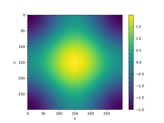
In this example the next block of code produces some plotable data. Code is executed, figure is saved and then code is presented next, followed by the inlined figure.

x = np.linspace(-np.pi, np.pi, 300)
xx, yy = np.meshgrid(x, x)
z = np.cos(xx) + np.cos(yy)

plt.figure()
plt.imshow(z)
plt.colorbar()
plt.xlabel('$x$')
plt.ylabel('$y$')

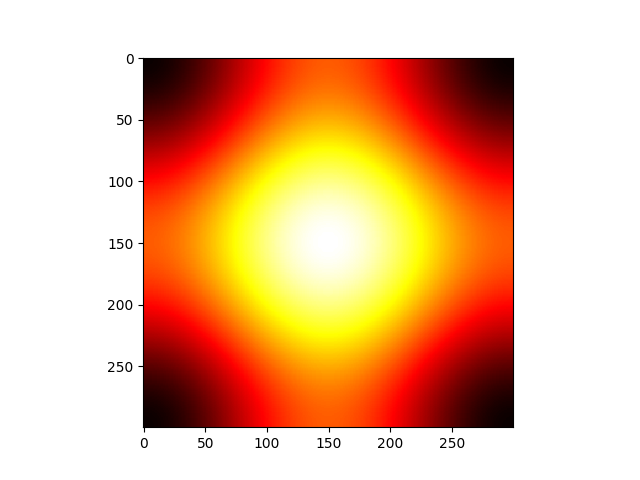
Again it is possble to continue the discussion with a new Python string. This time to introduce the next code block generates 2 separate figures.

plt.figure()
plt.imshow(z, cmap=plt.cm.get_cmap('hot'))
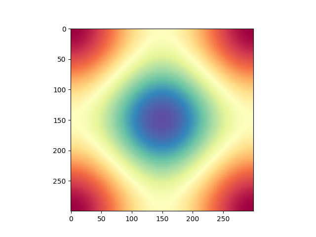
plt.figure()
plt.imshow(z, cmap=plt.cm.get_cmap('Spectral'), interpolation='none')

• 
• 

There’s some subtle differences between rendered html rendered comment strings and code comment strings which I’ll demonstrate below. (Some of this only makes sense if you look at the raw Python script)

Comments in comment blocks remain nested in the text.

def dummy():
    """Dummy function to make sure docstrings don't get rendered as text"""
    pass

# Code comments not preceded by the hash splitter are left in code blocks.

string = """
Triple-quoted string which tries to break parser but doesn't.
"""

Output of the script is captured:

print('Some output from Python')

Out:

Some output from Python

Finally, I’ll call show at the end just so someone running the Python code directly will see the plots; this is not necessary for creating the docs

plt.show()

You can also include inline, or as separate equations:

You can also insert images:

Total running time of the script: ( 0 minutes 0.064 seconds)